Sizing Guide
Introduction
OpenIO SDS is a highly flexible solution that allows users to build storage infrastructures that can respond to the most demanding requirements, both in terms of scalability and performance. In this section, we discuss the best practices for configuring an OpenIO cluster on x86 servers depending on use case, performance, and security requirements.
OpenIO SDS is supported on physical and virtual environments, but production clusters are usually deployed on physical nodes, due to their better efficiency and lower costs; this is particularly true for the storage layer. The access layer (S3/Swift services) can be deployed as physical or virtual machines depending on user requirements.
OpenIO SDS 18.10 can be installed on x86 servers compatible with Ubuntu 16.04 and Centos 7.
Cluster Layout
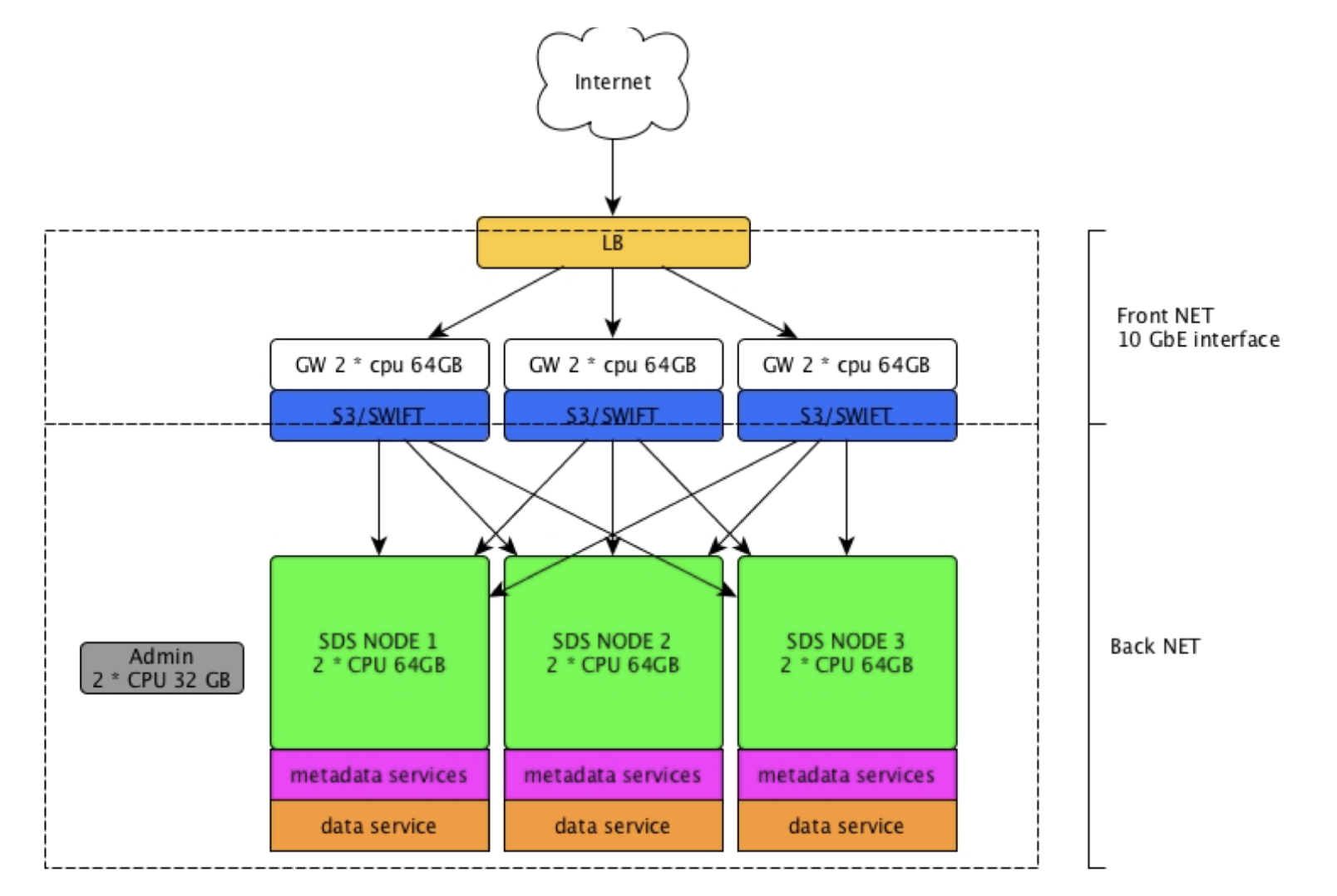
There are two types of supported production layouts:
- Simple configuration: each node provides front-end and back-end services. This configuration is very easy to deploy, scale, and maintain over time, with each additional node adding resources to the whole cluster. It is suitable for private networks and enterprise use cases, or in any other environment that doesn’t require granular scaling, strong multi-tenancy, or strict security policies. This type of configuration is cost effective for small clusters, but it is less efficient in large scale deployments, and could lead to higher costs over time.
- Split configuration: here, the access layer is separated from the storage layer. This cluster layout is more complex to deploy and maintain, but presents many advantages regarding security and efficiency. By separating the access layer from the rest of the cluster, it is possible to deploy front-end nodes directly on public networks (DMZ) while reducing the attack surface. These services are stateless and have a small number of open TCP/IP ports. Front-end nodes and back-end nodes have different characteristics in terms of CPU, RAM, network, and disk usage, and the separation increases the number of use cases, workloads, and effective multi-tenancy supported by the cluster. This type of configuration also allows the creation of multiple access points to separate traffic from private and public networks. For all the above reasons, this configuration is best suited for large scale deployments, service providers, and any other application where security is a main focus.
A simple cluster in the private network and a front-end layer in the DMZ is also supported.
CPU requirements
OpenIO SDS has a lightweight design. It can be installed on a single CPU core with 400MB RAM, but in production systems the minimum supported CPU has 4 cores. Intel CPUs with ISA-L support are required for erasure coding and compression; otherwise the performance impact is quite severe and a larger number of cores will be needed.
In the storage layer, the number of cores for each node has to be calculated by looking at the expected traffic generated by the node.
Storage layer
- For cold data and archiving workloads, CPU is less important, and a single 8-core CPU node is sufficient for a 90-disk server.
- In uses cases with small objects, such as for email storage, a small capacity node (12-24 HDDs) requires 2 10/16-core CPUs.
- For use cases that require high throughput, such as video streaming, a medium/large size node (48-90 HDDs) requires 2 8/12 CPU cores.
Front-end access layer
This type of node requires more CPU and RAM, as erasure coding, data encryption, and data chunking are usually computed at this level.
- For cold data and archiving workloads, CPU is less important, and a single 8-core CPU node is sufficient.
- In uses cases with small objects, such as for email storage, 2 10/16-core CPUs are required.
- For use cases that require high throughput, such as video streaming, 2 8/12 CPU cores are required.
- Erasure coding and compression, with ISA-L support, require an additional 10% of CPU power. Without ISA-L, 50% more CPU power is needed.
By adding up the number of CPU cores required for the front end and back end, it is easy to find the right number of cores needed for each node for simple layout configurations.
| Workload | Node capacity | Storage node | Access node | Single node |
|---|---|---|---|---|
| Cold data | 60-90 HDDs (0.5-1PB) | 8 | 8 | 16 |
| Small files frequent access | 10-24 HDDs (80-300TB) | 10-16 | 10-16 | 20-32 |
| Large files high throughput | 48-90 HDDs (0.5-1PB) | 8-12 | 8-12 | 16-24 |
RAM
Even though OpenIO SDS can run with a small amount of RAM, any additional resources improve performance because SDS leverages caching mechanisms for data, metadata, and other internal services.
The minimum RAM configuration for any type of cluster node is 8GB, but 16GB is highly recommended. Storage nodes use RAM primarily for caching metadata and data chunks. If the same data and metadata are frequently accessed, more RAM is recommended. Very small objects, less than 1MB in size, benefit the most from larger RAM configurations.
Storage layer RAM configuration
- For cold data and archiving workloads, large RAM configurations don’t offer any benefit. A large 90-disk server can be configured with 64GB of RAM.
- In uses cases with small objects, such as for email storage, a small capacity node (12-24 HDDs) requires more RAM: 32-64GB is usually the recommended configuration.
- For use cases that require high throughput, such as video streaming, a medium/large capacity node (48-90 HDDs) can take advantage of large caches, and 128GB is recommended.
Frontend access layer
This type of node is CPU and RAM heavy, since erasure coding, data encryption, and data chunking are usually computed at this level.
- For cold data and archiving workloads, 8GB of RAM is enough in most cases.
- In use cases with small objects, such as for email storage, RAM can bring a huge speed boost, and 32-64GB configurations can increase overall performance.
- For use cases that require high throughput, such as video streaming with large files, large RAM configurations are unnecessary; most of the caching is provided by the storage layer, and 32GB is usually accepted as a standard configuration in most scenarios.
By adding up RAM needs for the front end and back end, it is easy to find the right amount of RAM needed for each node for simple layout configurations.
Examples
| Workload | Node capacity | Storage node RAM | Access node RAM | Single node RAM |
|---|---|---|---|---|
| Cold data | 60-90 HDDs (0.5-1PB) | 64GB | 16GB | 80GB |
| Small files frequent access | 10-24 HDDs (80-300TB) | 32-64GB | 32-64GB | 64-128GB |
| Large files high throughput | 48-90 HDDs (0.5-1PB) | 128GB | 32GB | 160GB |
Storage
Flash memory
Flash memory is not mandatory, but it speeds up metadata searching and handling. It is usually recommended to add 0.3% of flash memory capacity to the overall data capacity. This number could be increased to 0.5% when the system is configured for very small files with a large quantity of metadata.
All-flash configurations are fully supported and, in this case, there is no need to separate metadata from data.
Storage Node Capacity
OpenIO SDS supports node capacities that range from one disk up to the limit of the largest servers available on the market (90-100 disks). The most common disk type used with OpenIO SDS is the 3.5” LFF with SATA interface. Disks with different capacities can be mixed in the same node. SMR (shingled magnetic recording) drives are not currently supported in production environments.
Nodes with different capacities are supported in the same cluster, but CPU/RAM/FLASH/DISK ratios should remain similar to maintain consistent levels of performance.
The net node capacity depends on the data protection schemes applied to the data, and whether it is compressed. As a general rule, formating and file system allocation add a 10% overhead to the original disk capacity.
Network
Any type of Ethernet network is supported. OpenIO SDS can run on single-port configurations, but this is usually done only for testing and development.
1Gbit/s Ethernet is supported for deep archive solutions, but in all other use cases, 10Gbit/s ports are mandatory. Higher speed networks are also supported.
For production environments, all front-end nodes should be accessible from at least two network paths for redundancy and load balancing. Front-end nodes should be equipped with two additional ports for back-end connectivity to separate north-south traffic and allow the enforcing of stronger security policies.
A private, redundant network for east-west cluster traffic is highly recommended for storage nodes. Access layer nodes access this network through their back-end ports.
In a simple layout, with front-end and back-end nodes collapsed, the nodes are connected directly to the network. Though a single dual-port connection is supported, it is strongly recommended to separate front-end and back-end traffic on two separate, redundant networks.
An additional, private, 1Gbit/sec network is necessary to connect all the nodes of the cluster for monitoring and management. Hardware management (IPMI or similar protocols), as well as OS and SDS management ports, can all be part of this network.
Load balancing
The front-end access layer is stateless, and doesn’t require any connection persistency or complex load-balancing protocols. Supported load-balancing solutions include HA-Proxy, and other third-party commercial load balancers with the HTTP protocol enabled.
Admin console configuration
An administration server is mandatory for production environments. It collects cluster logs, runs analytics, and provides the WebUI dashboard. This server could be physical or virtual, and must be connected to the monitoring and management network of the cluster.
Admin console configuration example:
- 1 x 8-core CPU
- 32GB RAM
- Boot disk
- 200GB SSD storage for storing logs and running analytics jobs
Tuning Services
meta0/meta1: Size the top-level index
In OpenIO SDS, the directory of services acts like a hash table: it is an associative array mapping unique identifiers to a list of services. Each unique ID corresponds to an end-user of the platform.
Our directory of services uses separate chaining to manage collisions: each slot of the top-level index points to an SQLite database managing all the services with the same hash. The top-level hash is managed by the meta0 service, while each slot is a database managed by a meta1 service.
So, how should the top-level index in meta0 be dimensioned? In other words, how many meta1 shards do you need? It will depend on the number of items you plan to have in each meta1 base, as there is one item for each service linked to an end-user.
Note
We recommend that you stay below 100k entries per SQLite file, and below 10k entries is a good practice.
| Digits | Slots | Behavior |
|---|---|---|
| 4 | 65536 | good for huge deployments (> 100M linked services) |
| 3 | 4096 | good up to 100M linked services |
| 2 | 256 | Advised when less then 64k, e.g. for “flat namespaces.” |
| 1 | 16 | minimal hash, only for demonstration purposes and sandboxing. |
| 0 | 1 | no-op hash, only for demonstration purposes. |
meta*: How many sqliterepo services
sqliterepo is software that manages a repository of SQLite databases, a cache of open databases, and a lock for each database. This software is used is the meta0, meta1, meta2, and sqlx services.
While there is no limit to the total number of databases currently held by the repository, the number of active databases should be low enough to fit in the current cache size.
As a default, the maximum number of databases kept in cache is 1/3 of the maximum number of open files allowed by the server, i.e. the RLIMIT_NOFILE fields of the getrlimit(), on the value that ulimit -n will return.
Note
for a given type of service based on sqliterepo, you should deploy enough services to have the active part of your population (of data) kept open and cached.
Zookeeper: Standalone services
With small demonstration or sandbox deployments, you won’t need to precisely dimension your Zookeeper instance. However, the general [Zookeeper administration guide](https://zookeeper.apache.org/doc/r3.4.12/zookeeperAdmin.html) might help you.
Zookeeper: Garbage collection
Make sure that Zookeeper doesn’t hang for too long while collecting garbage memory, and use the best GC implementation possible.
Note
-XX:+UseParallelGC -XX:ParallelGCThreads=8
Zookeeper: jute.maxbuffer
When the Zookeeper client is connected to the Zookeeper cluster, it sends heartbeat messages that refresh all the ephemeral nodes’ metadata, thus extending their TTL. The information is transactionally replicated to all the nodes in the cluster, and the transaction to do so will include the client connection. jute.maxbuffer is the maximum size allowed for the buffer in such an intra-cluster replication.
The problem you encounter is that the transaction includes the client’s connection, so that if the transaction fails, the connection with the client is reset by the cluster’s node. But the FSM (internal to the client) won’t enter in DISCONNECTED state and the application won’t be able to react to that situation. An insufficient buffer size is a well-known cause for transaction failure. The symptom is a client app continuously reconnecting to the Zookeeper cluster, with the service consuming 100% of CPU (in the ZK background thread).
The value is configured as a system property on the Zookeeper CLI using the
-Djute.maxbuffer=... option.
Note
when Zookeeper is used by OpenIO SDS, each ephemeral node requires approximately 150 bytes of metadata (110 for its name, 20 for the metadata, and 20 for the codec itself).
The default value for the buffer size is set to 1048576, and this lets you manage ~7,900 ephemeral nodes, or ~7,900 active databases on the server.